Analytical and Monte Carlo noise

Sweep a depolarizing rate on a 3-qubit GHZ state and compare Maestro’s two fast ways to estimate expectation values under Pauli noise.

import numpy as np

import maestro
from maestro.circuits import QuantumCircuit

qc = QuantumCircuit()
qc.h(0)
qc.cx(0, 1)
qc.cx(1, 2)

rates = np.linspace(0, 0.1, 11)
analytical, monte_carlo = [], []

for p in rates:
    noise = maestro.NoiseModel()
    noise.set_all_depolarizing(num_qubits=3, p=p)

    exact = maestro.noisy_estimate(qc, ["XXX"], noise)
    sampled = maestro.noisy_estimate_montecarlo(
        qc, ["XXX"], noise, noise_realizations=500, noise_seed=7
    )
    analytical.append(exact["expectation_values"][0])
    monte_carlo.append(sampled["expectation_values"][0])

for p, a, m in list(zip(rates, analytical, monte_carlo))[::5]:
    print(f"p={p:.2f}  analytical {a:.3f}  Monte Carlo {m:.3f}")

p=0.00  analytical 1.000  Monte Carlo 1.000
p=0.05  analytical 0.813  Monte Carlo 0.728
p=0.10  analytical 0.651  Monte Carlo 0.516

• noisy_estimate runs the circuit once without noise and damps each expectation value analytically. It costs nothing extra.

• noisy_estimate_montecarlo injects random Pauli errors after every gate and averages over many noisy runs, so noise builds up with circuit depth.

Show code cell source

Hide code cell source

import matplotlib.pyplot as plt

SURFACE, INK, MUTED, GRID = "#fcfcfb", "#0b0b0b", "#52514e", "#e4e3df"
BLUE, ORANGE = "#2a78d6", "#eb6834"

fig, ax = plt.subplots(figsize=(7, 4), facecolor=SURFACE)
ax.set_facecolor(SURFACE)

ax.plot(rates, analytical, color=BLUE, linewidth=2, label="Analytical (noisy_estimate)")
ax.plot(rates, monte_carlo, color=ORANGE, linestyle="none", marker="o", markersize=7,
        markeredgecolor=SURFACE, markeredgewidth=1.5, label="Monte Carlo (noisy_estimate_montecarlo)")

ax.annotate("Analytical", (rates[-1], analytical[-1]), xytext=(8, 0),
            textcoords="offset points", va="center", color=INK)
ax.annotate("Monte Carlo", (rates[-1], monte_carlo[-1]), xytext=(8, 0),
            textcoords="offset points", va="center", color=INK)

ax.set_title("⟨XXX⟩ on a 3-qubit GHZ state", loc="left", color=INK)
ax.set_xlabel("Depolarizing probability p", color=MUTED)
ax.set_ylabel("Expectation value", color=MUTED)
ax.set_xlim(0, 0.118)
ax.set_ylim(0, 1.05)
ax.grid(axis="y", color=GRID, linewidth=1)
ax.set_axisbelow(True)
ax.tick_params(colors=MUTED)
for side in ("top", "right", "left"):
    ax.spines[side].set_visible(False)
ax.spines["bottom"].set_color(GRID)
ax.legend(frameon=False, loc="lower left", labelcolor=INK)
fig.tight_layout()

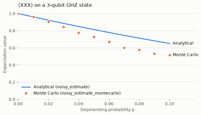
The Monte Carlo curve falls faster. A depolarizing channel with probability p scales a Pauli expectation value by 1 − 4p/3 each time it hits a qubit the observable acts on. The analytical mode applies that factor once per qubit, three times for XXX. Monte Carlo applies it after every gate, and five gate locations here touch a qubit the observable depends on:

p = rates[-1]
print(f"analytical  {analytical[-1]:.3f}   (1 - 4p/3)^3 = {(1 - 4 * p / 3) ** 3:.3f}")
print(f"Monte Carlo {monte_carlo[-1]:.3f}   (1 - 4p/3)^5 = {(1 - 4 * p / 3) ** 5:.3f}")

analytical  0.651   (1 - 4p/3)^3 = 0.651
Monte Carlo 0.516   (1 - 4p/3)^5 = 0.489

Use the analytical mode to screen many circuits quickly, and Monte Carlo when the depth of the circuit matters. Noise and error correction covers every noise mode.